Full-wave simulation extends the range and depth of lens analysis

In addition to the optical lenses found in cell phones, laptop computers, and more, we are surrounded by items processed through optical lenses every day. For example, many of the logos and other graphics seen on hardware devices, including cell phones and computers, are inscribed by a laser, or cut out by a high-power laser, in which case a laser beam had passed through many lenses. The same is true for food package date markings, markings on medical devices, and the so-called jamb stickers seen on car doors. As a result, we indirectly benefit to a great extent from computational lens analysis, without even knowing it.
Before such lenses (see Fig. 1) are used in the real world, a number of computer simulations are typically performed. While simulation does not replace testing, it can help reduce the number of prototypes needed and also provide valuable insight to conduct better experiments. For the simulation of lenses, different methods are available, ranging from traditional lens-design methods to simulations that solve the full Maxwell’s equations. But what might go into the decision to perform a lens simulation using one method over the other?
Design vs. analysis
For the purpose of this article, lens simulation can be divided into two categories: design and analysis. Design here means optimizing a lens for a particular application, whereas analysis means gaining a deeper understanding of what is going on in the lens system.
For lens design, one tries to find an optimal shape of a lens so that it delivers the beam in a desired way; put another way, to make sure the lens focuses or diverges the beam appropriately. The goal of lens design is usually to minimize the optical aberration. Simulation can be used to achieve an optimal lens design, and this is a standard application of optics simulation. For the purpose of lens design, a simulation is usually carried out by a ray-tracing method for reasons of computational efficiency.
In a ray-tracing simulation, the electromagnetic waves are approximated by rays. The drawback of this approach is that diffraction effects are not included. However, in many cases, understanding the diffraction effects is not critical for the design. When diffraction effects are important, wave-optics methods that solve for the full set of Maxwell’s equations without inherent approximations, other than the numerical ones required to fit the simulation in digital form on a computer, are used. When does one use wave optics instead of ray tracing for lens simulations? As it turns out, it is useful for both design and analysis.
Wave optics for lens design. In lens design, one of the important characteristics of the lens is the spot size. Ray tracing cannot simulate a focused beam because it is the result of diffraction effects. The detailed simulation of diffraction requires a full-wave optics simulation. To cope with this, ray tracing software often comes with some wave optics simulation tools, such as Fourier transformation and methods based on Huygens theorem and Fresnel diffraction. These three methods are sometimes collectively called physical optics. The formulas used are derived from an approximate theory and typically find a scalar electromagnetic field solution, which is good enough to design the beam size in many cases.
Wave optics for lens analysis. In lens analysis, physical optics may be adequate, but sometimes a more rigorous theory—specifically, Maxwell’s equations—are needed to obtain the full vector representation of the electromagnetic fields. This methodology is sometimes called the full-wave method. High-numerical-aperture lenses require a full-wave approach to be accurately analyzed; the physical-optics methods are not applicable for analyzing fast lenses.
When polarization matters or when the material has some anisotropic properties, a full-wave analysis is needed instead of scalar approximations. It is rare that a lens itself has such complicated properties, but it is also rare that the system being analyzed consists of only a single lens; several other optical components are usually involved. If so, it may be best to simulate not only the lens, but also the surrounding optics together with the lens by the full-wave method if possible. Historically, full-wave methods were frequently so computationally demanding that they were impossible to use in practice.
Physical optics vs. full-wave optics
There are two underlying differences between physical optics and full-wave simulations.
Propagation or domain solution. In the physical optics case, once the field is known in one plane, the method can calculate the field in another plane wherever it is; that is, it does not require the information between the two planes as long as the space between them is uniform. Therefore, it does not need a volumetric mesh in its computational domain.
On the other hand, the full-wave approach needs to solve for Maxwell’s equations in the entire domain. A very powerful numerical method for this purpose is the finite-element method, in which the domain is meshed; it is subdivided into small elements having a simple shape. The maximum mesh element size is limited to a fraction of the wavelength to satisfy the Nyquist criterion. The shorter the wavelength, the smaller the finite element mesh element size. A smaller element size means a greater number of finite elements are needed and with that comes greater computational resources in terms of computational time and memory.
Unidirectional or bidirectional. The physical optics methods typically find an outgoing wave field as a solution neglecting any reflections. This is how the physical optics formulas are derived. Compared to this, the full-wave method finds a solution that automatically includes reflections if there are any. If there are any material interfaces in the simulation model, Maxwell’s equations will not give an out-going wave field only, since it is not the real solution. The real solution is the coherently combined out-going wave field and the reflections from the material interfaces.
Lens simulation with the full-wave method
There are three reasons why lens simulations using the full-wave method are difficult.
Mesh. Keeping in mind that the full-wave approach requires the mesh and the mesh size needs to resolve the wave, one can immediately understand how difficult it is to simulate a lens with the full-wave method. If the size of the lens and the focal length are of millimeter-scale range, for example, the domain size can be a thousand times the wavelength. Then, the number of mesh elements will be in the billions, so a regular computer cannot handle it.
Refractive index. Usually, any optical component has a refractive index higher than one—say, 1.5. Then, the wavelength in the optical component is 1/1.5 times the wavelength, which is shorter than the wavelength in the vacuum. This again increases the number of mesh elements, thereby further increasing the computational demands.
Interference. Any optical component has material interfaces, where the Fresnel reflection takes place. There is a 4% reflection from a material surface of a refractive index of 1.5 for a beam of normal incidence. This reflection causes an interference with the incident beam, resulting in a fringe with the periodicity of one half of the wavelength. The mesh needs to resolve 1/2 times the wavelength. Combining with the refractive index effect, 1/3 times the wavelength needs to be resolved in the case of an index of 1.5; that is, the situation is three times worse for lens simulations than simulations in the open space, which is already difficult.
The beam-envelope method and AR coatings
From the above discussions, it sounds like it is almost impossible to simulate lenses. However, using the full-wave method, we have the following two remedies at our disposal:
The beam-envelope method. Instead of solving for the fast-oscillation electric field, the slowly varying envelope function can be solved for if the wave vector is known. This is called the beam envelope method. In this case, there is no theoretical approximation, but it is equivalent to solving Maxwell’s equations. In this formulation, the mesh needs to resolve the envelope function rather than the field itself. The number of mesh elements is greatly reduced if the envelope function is slowly varying, which is the case in practice for many lens simulations.
Antireflective (AR) coatings. Even with the beam-envelope method, the interference fringes do not give the designer a free pass because the envelope function is no longer slowly varying in the fringes. To remedy this, one can use an AR coating. It is possible to mimic a material interface with an artificial phase jump, which artificially generates a destructive interference with the incident beam and ends up with no fringes. Introducing this artificial AR coating can be motivated, since optical components are AR-coated in almost all practical cases.
COMSOL Multiphysics has these remedies available as built-in functionality. The Beam Envelopes interface of the Wave Optics Module is made with the beam-envelope formulation and includes the Transition boundary condition, which can be used as an AR coating. Full-wave lens simulations are therefore possible in a straightforward fashion by using a combination of the Beam Envelopes interface and the Transition boundary condition. It is possible to simulate slow lenses quite easily, whereas the simulation of fast lenses is more computationally demanding due to the fact that a finer mesh is needed. Fast lens simulations are still possible with a powerful-enough computer.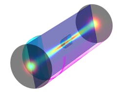
Full-wave simulations for multicomponent optical systems (see Fig. 2) have previously been out of reach. However, using the methods outlined in the article, an entire optical system, including lenses and other optical components, can be simulated, provided the AR coating approach is applicable. In addition, full-wave simulations make birefringence analyses possible so that it can be used for the simulation of not only lenses, but also liquid crystals or second-harmonic generation (SHG) optics, including the lenses. Full-wave simulations performed in this manner extend the range and depth of lens analysis.
ACKNOWLEDGEMENT
COMSOL Multiphysics is a registered trademark of COMSOL AB.
About the Author
Yosuke Mizuyama
Principal Engineer, COMSOL and Managing Director, COMSOL GK
Yosuke Mizuyama is formerly a principal engineer at COMSOL (Burlington, MA) and is now managing director at COMSOL GK (Tokyo, Japan).