Wave Optics: Beam-envelope method efficiently analyzes photonic components
When performing computations to answer questions surrounding the design of optical components, several different numerical methods can be useful. Which method to choose depends on the size of the component and the nature of the electromagnetic wave propagation. Very accurate general-purpose methods—so-called full-wave methods—are frequently used when designing micro- and nano-optical devices such as fiber-optic components, integrated photonics, and other waveguide-based components, whereas approximate methods such as ray tracing are needed when designing macroscopic lens systems. The following tutorial gives a quick background of the traditional methods and then demonstrates the newer beam-envelope method and its virtues in computational optics.
Full-wave methods
Computational high-frequency electromagnetics software uses an array of general-purpose numerical methods, including finite-difference, spectral, method-of-moments, and finite-element methods. Equipped with these tools, engineers can analyze propagating waves in optical structures with a minimal set of physical assumptions.
Over the years, these methods have been successfully applied to the analysis of important optical components such as optical fibers, directional couplers, and ring resonators. These general methods are sometimes referred to as full-wave methods. The name conveys that there are no inherent approximations other than those coming from creating a digital model by discretizing the piecewise continuous optical media. In this way, phenomena such as diffraction and low-order mode resonances can be captured by virtually arbitrary accuracy by simply refining the level of discretization.
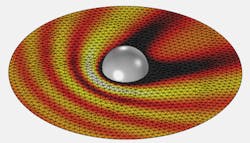
In the case of the finite-difference method, refining the level of discretization roughly means inserting more points in the computational domain so that the electromagnetic field can be represented in a smoother fashion, and similarly for the other methods. However, more discretization points means higher computational cost. For a 3D analysis, the number of discretization points, or elements, scale as the cube of the wavelength because of the Nyquist criterion (see Fig. 1). At least two sampling points per wavelength are needed in each coordinate direction, and even more in practice. The actual computational cost of the underlying numerical methods typically scales even worse, which implies that such full-wave methods are of limited use for cases where the relative number of wavelengths of the object of interest is large.
Approximate methods
In this class of methods, we find ray tracing, Gaussian optics, and beam-propagation methods. In special cases, these methods can be applied to much larger structures than full-wave approaches. For example, a centimeter-sized lens corresponds to tens of thousands of wavelengths of optical light in all directions.
In this case, a ray-tracing approach may be the best option. The approximations come at a cost-using a ray-tracing method typically implies that diffraction effects are neglected, as the rays are simply traveling in straight lines.
The beam-envelope method
A guiding structure in an optical system often has a well-defined and preferred propagation direction. In the language of mathematical physics, this means that there is a well-defined wave vector that is varying slowly, or even constant, in the direction of propagation. This is used in a relatively new computational method called the beam-envelope method, which is a full-wave method with some of the characteristics of an approximate method.
If we consider just the electrical field of a propagating wave, it has, in the most generic case, three components:
E = (Ex, Ey, Ez)
Each of the three field components can be a function of all three coordinate directions-for example, Ex = Ex (x, y, z). However, if there is a preferred direction of propagation-say, the z direction-then for an optically guiding component, this usually means that the field goes through many oscillations in the z direction while experiencing much slower variations in the x and y directions. Therefore, for a continuous single-frequency electromagnetic wave, we may choose to write the field as:
E = E1cos(ωt - kzz)
where ω = 2πf is the angular frequency, kzis the propagation constant in the z direction, z is the z coordinate, and E1 is the slowly varying part of the field.
Note that there may still be z variations in the slowly varying field. To clarify this, we may write it out more explicitly as:
E(x, y, z, t) = E1(x, y, z)cos(ωt - kzz)
This expression, or rather its complex-valued counterpart E = E1ej(ωt - kzz), can now be substituted into the full electromagnetic wave equations according to Maxwell. After some algebra, we will end up with an equation in only the slowly varying envelope field E1. In a strike of mathematical fortune, all terms involving the quickly varying factor ej(ωt - kzz) can be canceled from the equation. We just need to remember to multiply with this factor after our calculation to get back the true wave representation.
This fortunate cancellation of the quickly varying part of the field forms the basis of the beam-envelope method (see Fig. 2). This should not be confused with another related method, the beam-propagation method, which comes with additional simplifications and associated approximations resulting from throwing out some of the derivatives in the wave equation. On the other hand, the beam-envelope method comes with no approximation, but belongs to the class of full-wave methods.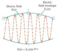
In which way does this mathematical trick help us? It all comes down to beating the Nyquist criterion. A major obstacle when using full-wave methods is that you have to sample the field with enough computational points, or nodes. If not, your computational result will be numerical garbage. By only solving for the slowly varying envelope field, the computational points can be sampled much more sparsely—at least in cases when there is a distinct direction of propagation, such as in an optical waveguide.
Variable and multiple directions of propagation
Being able to analyze long, slender structures with a more-or-less constant direction of propagation is important. It is fairly straightforward to see how to apply the beam-envelope method to such cases. However, a large class of guiding structures are bent in one or more directions. Can the method also be applied in these cases?
The answer is yes, if the structure is not too complicated. As long as the direction of propagation is slowly varying, the beam-envelope method is in good shape. To see how this works, we need to consider the full propagating fieldE = E1ej(ωt - kzz) again. Here, the direction of propagation is hardwired to be in the z direction. To handle a generic direction, we need to write this instead as E = E1ej(ωt - k·r), where k = (kx, ky, kz) is the propagation constant vector, which determines the wave's preferred direction of propagation, and r = (x, y, z) is the coordinate vector.
In practice, the dot product k · r = kxx + kyy + kzz is set equal to a spatially varying phase functionϕ(x, y, z) = k · r. The requirement of a slowly varying direction of propagation now gets translated into a slowly varying phase. For example, the circular part of a ring resonator of radius can be represented by a phase functionϕ = Rkparctan(y/x), where kp = 2π/(λp) is the propagation constant corresponding to the wavelength λp in the direction of propagation.
In this way, the beam-envelope method can be applied to a structure composed of simple shapes, where each component can be represented by a spatially varying phase factor corresponding to a locally preferred type of propagation. For example, a ring resonator consisting of one straight and one circular section can readily be analyzed this way by using one constant and one circular phase function, respectively (see Fig. 3). In a more general case, the phase function can be given by a look-up table that is a simple-enough function of the coordinate vector. In addition, by superimposing fields, two or more directions of propagation can be handled by supplying multiple sets of phase functions.
Applications in nonlinear optics
Nonlinear optical effects are often very weak and occur over long interaction lengths. Here, the beam-envelope method is useful. Self-focusing is one such nonlinear phenomenon—important from a laser engineering perspective—where the modification of the beam must be incorporated into the design. The effect may be seen, for example, in laser rods or glass components placed at a focal point. If the threshold for self-focusing is exceeded, the material is damaged. It is important to know the self-focusing threshold values for the materials used in the design. Self-focusing occurs in dielectrics, like optical glasses and laser rod materials, such as Nd:YAG.
Other nonlinear effects for which the method is applicable include second-harmonic generation, sum- and difference-frequency generation, parametric generation and amplification, and self-phase modulation.
The beam-envelope method extends the use of full-wave methods to previously unattainable model sizes. It fills a gap between computationally heavy, but accurate, traditional finite-element/difference methods and fast-to-compute ray-tracing methods. Successes within nonlinear optics show the method's applicability for real-world design tasks. In the future, we will most likely see this method being combined with traditional full-wave and ray-tracing methods to reach new frontiers in computational optics.