SOFTWARE & COMPUTING: Optical software models partially spatially coherent beam propagation

RICH PFISTERER
Most optical engineers can adequately perform their engineering tasks by assuming that the light propagating through their systems is either totally spatially incoherent or coherent. For example, an illumination designer working with light-emitting diodes (LEDs) can accurately model the distribution of LED light on a display by considering each ray as a delta function carrying with it some amount of power; the total power incident on the display is therefore the incoherent summation of all rays intersecting the surface. Likewise, an engineer propagating a laser beam through a system will calculate the correct energy distribution on target by considering that the beam is coherent. Both calculations have been widely available in commercial optical design and engineering software for more than 30 years.
However, there are numerous common applications that exploit partially spatially coherent light, and so assuming that the light is either totally coherent or totally incoherent would yield a completely incorrect answer. In photolithographic applications, for example, the correct results can be obtained only if the light is assumed to be partially spatially coherent. Astronomers using stellar interferometers take advantage of partial spatial coherence to measure the diameters of stars. And microscopists use partial spatial coherence to optimize resolution.
One of the common misconceptions about partial spatial coherence is that it is somehow the "average" of the results obtained by incoherent and coherent propagation. Nothing could be further from the truth. Consider a photolithographic system working at a wavelength of 193 nm. The diffraction-limited core diameter of the Airy disk produced by a system working at f/0.5 is 235.5 nm, and yet structures on the order of 45 nm are routinely fabricated! Clearly, partial spatial coherence has unique properties not shared with its more common cousins.
Synthesizing partially spatially coherent light
Mathematical theories for partially spatially coherent beams are considerably more complex than conventional coherence theory.1,2 However, distilled to the basics, partially spatially coherent light—like Gaussian beams—can be constructed and propagated using the same analytic tools with which we are already familiar. That is, even though partially spatially coherent light is not the "average" of incoherent and coherent light, it can be modeled in software as the incoherent addition of coherent light from a distribution of spatially separated sources, each with a different wavelength.
Consider a straightforward example using a diffractometer—an optical system that demonstrates the interference of partially spatially coherent fields (see Fig. 1).3 An aperture σ of diameter 2ρ located at the focus of lens L1 is populated with a distribution of coherent point sources radiating towards lens L1; the Airy core of each point source is small compared to the aperture diameter. Consequently, aperture σ1 acts like an extended incoherent source by superposition.
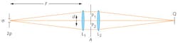
The diameter of aperture σ and how it is populated (sampled) by rays determines the coherence state of the system. If the diameter of the aperture were reduced to nearly zero and a single point source were present, then a single spherical diverging wave would impinge on lens L1 and we would have a purely coherent system. But if the aperture were of arbitrary diameter and populated with incoherent rays, then we would have an incoherent system. For a partially spatially coherent system, we want to create a source that is quasi-monochromatic and extended (and therefore incoherent), but filled with coherent point sources.
Since it is arbitrary, we can control the area in the plane of lens L1 over which the field is coherent (to whatever level necessary) by properly setting the diameter of aperture σ. From a derivation for the degree of coherence function |μ12| and assuming at most a 12% drop in coherence over that area, we find that the optimum diameter 2ρ for aperture σ for a partially spatially coherent system is given by
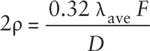
Here, λave is the average wavelength, F is the focal length of lens L1, and D is the diameter of the circular area. Note that while there are limitations imposed on the spectral bandwidth that are related to the coherence length of the source and the focal length of the lens L1, most engineers would not normally be restricted by them.
By the van Cittert-Zernike theorem, there is a correlation between the fields at any two points on the first surface of lens L1 that can be quantified by performing two-beam interferometry. Consider two pinholes P1 and P2 in plane A in the collimated space following lens L1. For simplicity, assume that the pinholes are equally spaced from the optical axis and that their total separation is d. Lens L2 focuses the light onto output plane Q where the two beams interfere to produce a fringe pattern. By measuring the fringe visibility, we can compute the degree of coherence.
A numerical example
Theory predicts that the degree of coherence function |μ12| is given by
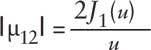
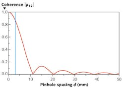
In this equation, u = 2πρd/(λaveF). For the sake of a numerical example, assume that ρ = 0.045 mm, F = 1505.42 mm, and λave = 0.546 μm. As a function of the pinhole separation, the predicted coherence function can be computed (see Fig. 2). The blue line indicates the area over which the field at lens L1 is approximately coherent. Note that the degree of coherence becomes progressively smaller as the pinhole spacing is increased, and in the limit we have a completely incoherent summation.
The irradiance distribution E(θ, d) at the point Q(θ) has an analytic solution given by
Here, v = 2πa sin(θ)/λave, δ = 2πd sin(θ)/λave, and β12(u) = 0 for 2J1(u)/ u > 0 and π for 2J1(u)/ u < 0.
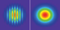
The computed interference patterns for pinhole separations of 6.5 mm and 20.34 mm correspond to |μ12| values of 0.5 and 0.002, respectively (see Fig. 3). In these calculations, 250 point sources uniformly spanning a 4 nm spectral bandwidth filled the aperture.
Since most commercial optical software already has the ability to propagate coherent and incoherent fields through optical systems, a relatively simple extension to incoherently sum the coherent fields from multiple point sources would offer the capability to propagate partially spatially coherent light.
REFERENCES
1. M. Born and E. Wolf, Principles of Optics (1970).
2. E. Wolf, Introduction to the Theory of Coherence and Polarization (2007).
3. B.J. Thompson and E. Wolf, "Two Beam Interference with Partially Coherent Light," J. Opt. Soc. Am., 47, 895–902 (1957).
Rich Pfisterer is president of Photon Engineering, 440 South Williams Blvd., Suite 106, Tucson, AZ 85711; e-mail: [email protected]; www.photonengr.com.
More Laser Focus World Current Issue Articles
More Laser Focus World Archives Issue Articles