Multiscale optical simulations pose unique challenges
For engineers working with optical simulation, the best choice of numerical method depends on the optical size of the model geometry. For a simulation domain a few wavelengths across, the finite element method is widely used. For a geometry spanning a large number of wavelengths, ray tracing is a popular alternative.
Optical simulations combine vastly different length scales, which includes high-aspect-ratio geometries as well as wavelength-scale components embedded in much larger systems or environments. There are unique challenges in combining simulations over multiple length scales based on different numerical formulations.
Wavelength and optical size
Electromagnetic waves, and the media through which they propagate, appear in a tremendous range of different sizes. We routinely encounter visible light waves (400–750 nm, where 1 nm = 10-9 m); FM radio waves (3 m); and nearly everything in between. When considering the propagation of electromagnetic radiation, we consider the surroundings to be optically large if the space dimensions are all significantly greater than the wavelength of the radiation we are studying.
For example, when studying how visible light is focused by the human eye, we can say the lens of the eyeball is optically large because it is about 10,000X thicker than the wavelength of visible light.
The concept of optical size is essential to choosing a formulation for numerical simulation of electromagnetic waves. Engineers working with simulation are constantly tasked with balancing accuracy against computational cost; we try to produce a model that best represents real-world behavior, but it must be within the time constraints of our assignment and with the limited computational resources at hand.
Finite element method
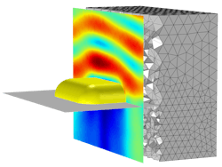
The finite element method (FEM) is a popular technique for modeling wave propagation over relatively short distances. In FEM, the model geometry is partitioned into small regions—mesh elements—and then a system of equations is solved numerically over these elements (see Fig. 1).
There are several different ways to model electromagnetic waves with FEM. There is the so-called full-wave approach, in which we solve Maxwell’s equations for the electric field directly. This full-wave approach can represent real-world phenomena very accurately because it does not make too many simplifying assumptions. It can faithfully reproduce wavelength-scale behaviors such as diffraction and interference, which significantly impact the operation of nanophotonic devices.
The main drawback of the full-wave solution is that the mesh must be fine enough to resolve individual oscillations of the electric field, so the simulations require more time and RAM to solve as the geometry size is increased. Therefore, this method is best suited for a model geometry that does not exceed a few wavelengths in all directions.
Ray tracing
Ray tracing is a simplified way to handle light propagation when the geometry is optically large, meaning the geometry spans a very large number of wavelengths in each direction (see Fig. 2). Instead of resolving individual waves on a very fine mesh, we represent the light as rays that can reflect and refract at boundaries between different media.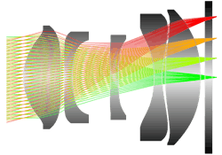
Wavelength-scale phenomena such as diffraction are usually neglected. If a collimated beam of light hits an obstruction, in a ray optics model we would not see Fraunhofer diffraction patterns—just distinct regions of light and shadow.
Modeling high-aspect-ratio geometries
Which method should we use if the geometry has one dimension that is comparable to the wavelength, but another dimension that is much longer? These high-aspect-ratio geometries are ubiquitous in fiber-optic cables and directional couplers.
One viable approach is the beam envelope method. Starting from the full-wave solution to Maxwell’s equations, in which the instantaneous electric field amplitude is resolved over each wavelength, we can apply a clever change of variables and instead solve for the amplitude of a slowly varying amplitude function. This relaxes the requirement from full-wave FEM that the mesh elements must be small enough to resolve individual wavelengths (see Fig. 3).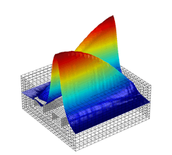
The beam envelope method is best suited for systems in which waves are constrained to propagate in one or two known directions, including in cables and directional couplers. These known directions of propagation are used to convert between the instantaneous and slowly varying amplitudes, which makes the beam envelope method possible. This method is less viable when light could propagate in many different directions at a single location—for example, a fluorescent lamp illuminating a room.
Submodeling
What happens if we have a very small object, comparable to a single wavelength, embedded in a much larger geometry? To understand a wavelength-sized object in detail, a very accurate approach like full-wave FEM is required, but the cost to mesh the open space around the object is most likely prohibitive.
A viable alternative here is to set up two models, using the output from one model as the input to the other.
Periodic substructures in multiscale models
Let us consider a diffraction grating, an optical component that is periodic (repeating) in one direction, where the period is usually comparable to the wavelength of visible light. When light hits the grating, it is reflected and transmitted in several different directions, known as diffraction orders.
The directions of the diffraction orders can be computed using a simple analytic formula that depends on the angle of the light hitting the grating and the period of the grating structure. However, this simple formula does not tell you the relative amplitudes of the different orders. For example, an Échelle grating is optimized to reflect most of the light in a high diffraction order; its microstructure usually consists of blazed (tilted) surfaces.
Another approach is to compute a full-wave solution of a single period of the diffraction grating using Floquet (periodic) boundary conditions (see Fig. 4). The full-wave model can accurately compute the transmittance and reflectance of each diffraction order, which can then be used as input to the ray optics model.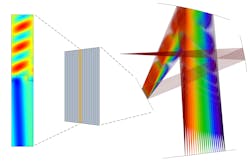
Submodeling with far-field radiation patterns
The final example we consider is primarily used at radio frequencies (RF) but will become more relevant at higher frequencies as devices continue to become smaller. A full-wave model of a radiating object, such as an antenna, can include a so-called far-field calculation — this uses the full-wave solution over a couple of wavelengths to compute the asymptotic limit of the electric field at very large distances from the antenna in all directions (see Fig. 5).
This far-field radiation pattern could also be used as input to a ray optics simulation; it basically becomes a directivity function that sets the amplitude and polarization of rays based on their initial direction. Altogether, this enables us to model antennas or scattering centers very accurately at the wavelength scale, and then use that information to predict how the emitted radiation will interact with other objects in the surrounding environment—perhaps tens of thousands of wavelengths away.
Looking forward
Optical devices appear in an immense range of optical sizes and aspect ratios. Through proficiency in several different numerical methods and the ways in which they can be coupled to each other, engineers specializing in optical simulation can create models that provide an ever-deepening understanding of the real world.
About the Author

Christopher Boucher
Lead Developer
Christopher Boucher is a lead developer at COMSOL. He received his BS degree in aerospace engineering and physics from Worcester Polytechnic Institute (WPI) before joining COMSOL in 2012.