White-light interferometry resolves sub-Angstrom surface roughness

FIGURE 1. The power spectral density (PSD) is created by taking a Fourier transform of the measured surface [1].

The demand for high-efficiency optics is driven by the need for more-powerful and more-sensitive instrumentation. Such instrumentation commonly requires extremely low surface scatter, very near 100% transmission or reflectivity, and high laser damage threshold values. For this reason, sub-Angstrom surface roughness has become a critical aspect of cutting-edge optical systems.

This article will explain the proper way to measure sub-Angstrom roughness and provide an overview of common instruments used for such applications. Specifically, this article will focus on the capabilities of white light interferometry and explain the necessary steps to push this measurement system to the level of performance required to properly analyze sub-Angstrom surface roughness.

Sub-Angstrom surfaces push the limits of surface topography instruments, which is why accurately measuring them is tricky. Two measurement systems used for this purpose, the white light interferometer (WLI) and the atomic force microscope (AFM), will be the focus of this article, but to offer a thorough understanding of sub-Angstrom surface roughness metrology, it is necessary to first understand power spectral density (PSD) and its relationship to the commonly used roughness value, root mean square (RMS).

Essentially, RMS is a simple algorithm used to determine a single value from a body of data, and the PSD illustrates that body of data in the form of a plot. Once raw data has been collected, a Fourier transform is applied to it, which separates the data into its respective spatial frequency components. In other words, this process will convert the data from spatial domain to frequency domain and describe the surface with a series of sine functions known as spatial frequencies. This process offers a very elegant way to analyze surface characteristics (see Fig. 1).

Power spectral density

The PSD plot (see Fig. 2) provides the relative strength of each roughness component as a function of spatial frequency and is very helpful for several reasons. First, if the surface has any structure to it, this structure will show up in the PSD plot as a data spike, which indicates a repeating pattern on the surface associated with a particular spatial frequency. For sub-Angstrom surfaces, no structure or pattern should be visible and the PSD graph should be more or less smooth.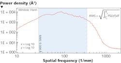

FIGURE 2. The instrument transfer function (ITF) and the PSD must be well understood, and the correct spatial frequency bandwidth must be applied to the data.

Second, the PSD indicates the measurement range of the instrument in terms of spatial frequencies. For example, the graph in Figure 2 shows a steep drop beginning around 400 cycles per millimeter. This is the point where the instrument’s ability to resolve detail becomes severely attenuated. Spatial frequencies past this point should not be included because the data is largely made up of signal noise and system error.

Third, the measured spatial frequency bandwidth defines the surface roughness value. Shown in equation form in Figure 2, integrating the spatial frequency bandwidth and taking the square root produces the RMS value. If the spatial frequency bandwidth is unknown, the roughness value will be undefined and largely meaningless.

Fourth, the spatial frequency bandwidth shows exactly what surface characteristics are being evaluated, which aids in the proper transfer of information and offers all parties involved the knowledge required to duplicate the measurement. For example, the light blue region in Figure 2 shows the spatial frequency bandwidth used to create the RMS value of a surface being evaluated—0.304 Å. This bandwidth is all the information required for an independent lab to confirm the measurement.

Spatial frequency bandwidth

The majority of the errors contained in our data reside in the far-right and far-left spatial frequencies (outside the light blue region). As a result, these frequencies have been excluded from the measured value. A further explanation of these errors requires knowledge of the instrument transfer function (ITF), which is essentially an evaluation of the instrument’s capabilities in terms of spatial frequencies. However, calculating this is a fairly complicated matter and the topic of another discussion.

By defining a meaningful spatial frequency bandwidth based on the instrument transfer function, the data becomes much more reliable. If not excluded, these outlying spatial frequencies would make differentiating instrument errors from real data virtually impossible. Taking these steps will increase the fidelity of the instrument, produce robust data, push the noise floor as low as possible, and ensure that the generated RMS value is accurate and verifiable.

With a proper understanding of how roughness values are created and defined, sub-Angstrom surface roughness metrology can be achieved. Both the WLI and the AFM are capable of evaluating spatial frequencies associated with surface roughness, have a noise floor low enough to measure sub-Angstrom surfaces, and will produce meaningful data. However, they are not at all equal in function or form, and in terms of spatial frequency range are quite different. The table shows a reasonable range of each instrument’s capabilities and illustrates their configurability.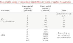

The WLI can be used with a variety of interferometric objectives, which will change the lateral resolution and field of view. This, in essence, allows the user to shift the spatial frequency range of the instrument. The AFM is configurable in a completely different way; the instrument collects a finite amount of data points as the stylus traces the surface. The spacing between these data points can be increased or decreased to change the resolution of the image and, as a result, change the spatial frequency range of the instrument.

Spatial frequency range

These features add a great amount of flexibility in terms of overall capability, but the spatial frequency range of an individual measurement will be much narrower than the total capacity of the instrument. The user will have to choose a meaningful range of spatial frequencies to evaluate, and if a larger range or bandwidth of spatial frequencies is required, data correlation will be necessary.

Notice the overlap in both instrument’s capabilities. This allows data correlation between the WLI and the AFM. It is entirely possible to use both instruments to extend the PSD plot, which if needed would allow a larger spatial frequency bandwidth to be evaluated. One might choose to do this if the range of spatial frequencies critical for a particular application fell between the two instruments.

The same instrument can achieve this as well, by correlating measurements from different instrument configurations. For example, by correlating data taken with the 50X and 100X objectives, we could create a spatial frequency bandwidth ranging from 25 to 1800 cycles/millimeter. This would allow a larger body of data to be examined and may offer a better prediction of performance in certain applications.

Which instrument is better depends on the range of spatial frequencies needing to be evaluated. It is generally accepted that applications in the visible range need not be analyzed beyond about 2000 cycles/millimeter, making the WLI ideally suited for this purpose. For applications in the UV, the higher spatial frequency capability of the AFM is more relevant. The AFM can also image the lower spatial frequencies (as shown in the table), but other factors must be considered when choosing the best instrument for a particular application.

For example, the AFM requires longer measurement times, which makes it more sensitive to environmental errors such as temperature fluctuation and vibration. For this reason, the AFM is more ideal for the controlled environment of a test lab rather than a factory floor. Also, the AFM uses a stylus that periodically needs replacing, while the WLI, being an optical measurement, has no disposable parts and is less maintenance-intensive.

Evaluating sub-Angstrom surfaces

To successfully measure sub-Angstrom surfaces, a relatively esoteric knowledge of these instruments must be understood. Just pushing the measurement button will most likely not produce meaningful data. Remember that evaluating sub-Angstrom surfaces pushes the limits of both the WLI and AFM, and because of this, steps must be taken to ensure the instruments’ optimal performance.

The ITF and the PSD must be well understood, and the correct spatial frequency bandwidth (illustrated by the PSD plot in Figure 2) must be applied to the data. If the roughness value requires verification by the customer or a third-party lab, the spatial frequency bandwidth that created it must be stated; the measurement cannot be properly duplicated without this information. This level of transparency offers all parties involved a complete understanding of exactly what has been measured, and is often the only difference between a good optical system and a great one.

REFERENCE

1. See https://bit.ly/EdmundRef1.