Interferometry: Three simple tests assess interferometer performance

Computer numerically controlled (CNC) polishing machines can produce almost any surface imaginable, and yet most interferometers in optical shops were architected in the 1970s and are not designed nor specified to measure CNC-polished surfaces.

So, how do you know if your interferometer supports your production requirements? How do you measure your interferometer performance to know it works as well as needed or as well as last year? Fortunately, for optical engineers armed with an intimate knowledge of interferometer architecture and evolution, three simple tests can assess whether or not your interferometer supports your specific process control needs.

Next-generation optics

Optical component manufacturing has radically changed since the turn of the century: CNC polishing now enables the manufacture of any surface shape from spherical to aspheric, freeform, and even phase plates. Each of these surfaces may start and at times will end with large deviations from a spherical surface, placing new demands on optical test & measurement equipment.

In an interferometer, surface deviations from spherical are seen as large wavefront slopes marked by areas of dense, closely spaced fringes. Any instrument's ability to measure these slopes is limited and in CNC-produced optics, spot polishing potentially creates localized errors termed mid-spatial frequency surface features that must be accurately measured and minimized.

Both fast and easy to use, the laser Fizeau interferometer has been the tool of choice for optical manufacturing since the early 1970s. An understanding of the evolution of interferometer design demonstrates why interferometers are trusted by the optics industry, what limitations can be present, and how they can be tested to ensure they are working properly.

Fizeau interferometer architecture

During the 1960s, the newly invented laser could easily create interference patterns between a test and reference surface. All interferometers were unique to each measurement configuration and required a PhD to align and operate, thereby limiting their production application. But this situation changed in the 1970s with the invention of the modular Fizeau interferometer architecture by Zanoni and Hunter, comprised of an interferometer and a reference optic and replacing the test plate as the primary testing method.

A few years later, limited by the technology of the day, Domenicali and Hunter created an optical system with a coherent testing section and incoherent imaging section.¹ The incoherent imaging was required to accommodate a low-resolution vidicon camera and a commercial television zoom lens so that small parts could be seen, as this was a visual-only system. Both the zoom and vidicon had multiple optical surfaces that created a confusing background of internal Fizeau interference patterns, requiring a rotating ground-glass surface to be added as a coherence scrambling intermediary component to suppress the confusion.

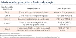
In the 1970s, no design considerations were made for phase-shifting interferometry (PSI) measurements, as PSI was being developed at the same time elsewhere. Interferometers containing a rotating ground glass and zoom lens are based on this design and are considered generation I (Gen I) or Gen II systems (see table).

Phase measurement

At Bell Laboratories, driven by the increased optical quality demands of the semiconductor business, Bruning and co-workers invented phase-measuring interferometry.² Pixel-by-pixel phase data was measured by varying the cavity length in a Twyman-Green interferometer, wherein four intensity frames were acquired at four phases.

Instead of visual or computerized fringe-tracing analysis where only global information was seen, the pixel-by-pixel acquisition allowed for higher-resolution correction and finer height measurements, launching the production of higher-quality optical manufacturing. This system was implemented at Tropel (now Corning Incorporated) in the late 1970s with a 32 × 32 pixel readout of a then state-of-the-art vidicon camera.

In the early 1980s, the zoom lens/diffuser disk Fizeau configuration interferometer was married to PSI, creating Gen II and III interferometers. From the early 1980s until 2000, the data acquisition system was the primary area of advancement in interferometry with faster computers, higher resolution cameras, and new acquisition, analysis, and display software. After 2000, Gen IV and V systems began to appear, driven by advances in optical manufacturing processes.

New interferometers, better measurements

In the early 2000s, optical manufacturing advanced significantly with the wider acceptance of CNC polishing, demanding improved interferometer performance. Based on localized or spot polishing, CNC optics require manufacturers to know where and how much to correct to minimize mid-spatial frequency errors.

For manufacturers wondering if old interferometer architectures will work for their applications, specification sheets often are of little help. Features such as zoom range or discrete magnification, or fixed imaging system with camera pixel count, are meaningless in themselves—what matters is the resolution and image distortion of the interferometer.

Historically, measurement repeatability has been the canonical interferometer performance parameter. Today, with vibration-tolerant data acquisition and 12-bit cameras, measurement repeatability is in the noise compared to other error sources like those caused by air turbulence or reference surface accuracy. Further repeatability, with many averages of nulled, extremely short plano cavities, does not reflect daily usage where most measurements have no averaging and use much longer cavities. So, what matters?

Just adding higher-pixel-count cameras will not help if the interferometer's optical design is a limiting factor. For instance, what is acceptable image distortion in a visual-only system is not sufficient to place a CNC machine in the correct spot. The ability to measure high slopes (many closely spaced fringes) is now needed to quickly start final polishing or to manufacture non-spherical surfaces.

Finally, when measuring parts that deviate from perfect, optical system or retrace errors limit system accuracy and thus limit the ability to meet manufacturing tolerances. Knowing how any interferometer measures up to these requirements can be described by three simple tests.

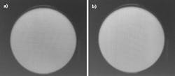
Test 1: Image resolution

Interferometric imaging systems, like photographic cameras, can be characterized by their modulation transfer function (MTF). Targets of finer and finer lines are imaged until the contrast falls below a threshold. But because interferometers measure wavefront phase and not intensity, a new function has been proposed called the Instrument Transfer Function (ITF).

The ITF test target has approximately 100-nm-tall features with various spatial frequencies present to determine the phase image resolution limit. There is industry discussion regarding the appropriate step heights because of nonlinear responses and target structure, plus some discussion as to whether ITF is a valid parameter.^3-4

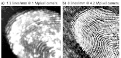
To avoid these difficulties, simply testing the MTF image quality is a good start. If an interferometer will not pass a simple visual MTF-type test, it will not pass an ITF test. Although a complicated MTF target could be developed, a simple test will often suffice:

1. Use your computer to create a pattern of black/white line pairs every millimeter over a 125 × 125 mm area large enough to be imaged by a 4 in. interferometer, and print this pattern on a stiff piece of paper.
2. Remove all reference optics (transmission flat or transmission sphere) from your interferometer and place the card approximately 200 mm in front of the aperture, perpendicular to the table so it can be imaged by the interferometer.
3. Shine a bright lamp on the card, observe the image in the data acquisition (view) camera, and, using the camera, adjust focus until the card is as sharp as possible.
4. Observe the sharpness and apparent image contrast that indicate the limits of resolution, looking carefully at the edges of the field of view (FOV) for line uniformity.

These problems can be inherent limitations in the optical system, or an indication of internal optical misalignments. Running these tests annually (or periodically) can be part of the interferometer's calibration test to confirm nothing has changed that requires repair or adjustment.

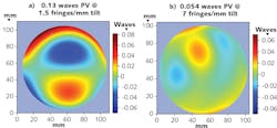
Test 2: Wavefront error at maximum measurable fringes

Measuring large differences between an optical surface and reference creates high-density interference fringes. With CNC polishing, the sooner correcting can begin, the faster the part can be completed—therefore, you need to measure the largest fringe differences possible. Our second test indicates the measurement accuracy of parts with large surface errors:

1. Place a transmission flat (TF) reference into the interferometer and adjust the tip and tilt on the front of the interferometer until the TF is aligned (return spot centered in the alignment target).
2. Mount a matching-sized reference flat in the test part mount and adjust the tip and tilt of the part mount until the spot is centered in the alignment cross hairs and fringes come into view.
3. Adjust the test part mount until the observed fringes fill the camera and appear to pulse uniformly, indicating that the cavity is nulled.
4. Use the interferometer software to acquire and save this reference result to a file for later subtraction.
5. Again using the test part mount, tilt the fringes in any direction until the fringes of increasing density appear to fade. At this point, take a measurement. If the phase data plot has no data loss, continue to increase the tilt in the same direction, one-quarter knob turn (or less) at a time, measuring after each turn until there is data loss (holes in parts of the data).
6. When data loss appears, repeatably back up one-eighth turn (or less), and try again until there is no data loss, indicating that these are the maximum measurable fringes for this interferometer.
7. Finally, subtract the reference result (step 4) from the data set with maximum measurable fringes.

An additional instructive step is to repeat this same measurement without changing the maximum tilt, but instead changing the focus position. Some imaging systems exhibit focus-position-induced errors when high slopes are encountered. This additional step can indicate how carefully you need to focus and the potential errors that can be induced.

Test 3: Maximum measurable fringes

To quantify the maximum measurable fringes, start with the results of the previous test. The maximum measurable fringes are found by observing the tilt results with the interferometer units set to fringes rather than tilt.

It is obvious that interferometer performance limits what types of optical components you can produce and how fast you can converge to meet specification and minimize mid-spatial frequency errors in CNC-polished components. If you cannot observe surfaces during the manufacturing process because of the presence of steep slopes, look for an interferometer with higher maximum fringe acceptance. Because measurement accuracy is the core parameter driving rapid convergence to the final figure and to meeting specifications, these simple tests can confirm that your interferometer is up to the challenge, especially if high slopes are considered.

REFERENCES

1. P. Domenicali and G. Hunter, U.S. Patent 4,201,473 (1978).

2. J. Bruning et al., Appl. Opt., 13, 11, 2693–2703 (1974).

3. E. Novak et al., "Transfer function characterization of laser Fizeau interferometer for high-spatial-frequency phase measurements," Proc. SPIE, 3134, 114–121 (Nov. 1997).

4. Y. Yashchuk et al., Opt. Eng., 50, 9, 093604 (Sep. 2011).