Optical Design: Downhill simplex algorithm optimizes luminaire designs

DAVID JACOBSEN

Optical engineers designing products that include integrated LEDs or light pipes must take into account myriad factors such as reflectivity and intensity, properties of surface materials, and other characteristics that improve the products' aesthetic or functional performance. In a rush to get products to market, project schedules are being increasingly compressed; as a result, compromises are often required.

This often means that product concepts are brought directly to prototype, which is a recipe for poor results. On occasion, design engineers use rudimentary optical simulation tools that produce illumination performance that's "good enough." Simply using brute-force processes to create a better design is computationally intensive, requiring thousands of hours to complete—an impractical approach that engineers won't likely perform more than once, if at all.

While computational power has dramatically increased over the years, the "black-box" approach for solving an optical problem, where the multidimensional merit function cannot be expressed in a closed-form solution, still requires massive, time-consuming numerical simulation. This is particularly true for a system that needs to be evaluated by the Monte-Carlo technique, which requires a large number of rays to produce an accurate evaluation.

The downhill simplex optimization method is a technique used by optical and illumination simulation software to automatically find an optimal solution. This method is considered a good approach for general optical-design cases. Its purely geometrical operation disregards the complexity of systems, using a single computation to determine the next step of the optimization, which makes it incredibly efficient for cases that require an evaluation using lots of ray tracing.

Although typically recognized as a local optimization method, by generating the initial simplex with a random process, the downhill simplex method can become a nonlocal concept and, therefore, acquires the ability to find a local minimum not necessarily closest to the starting position. Downhill simplex is particularly effective when designers are working with multiple elements within their design, such as reflectors, lenses, diffusers, LED arrays, and other optical components.

How downhill simplex works

The downhill simplex method is a nonlinear optimization that starts with an initial geometric figure—or simplex—that is defined by N + 1 points. The simplex is multidimensional, meaning that it's a polytope with set dimensions for its volume, faces, edges (also known as line segments), and vertices. By changing the values of these interconnected functions, the method interactively changes the shape of the simplex until it converges into the best practical solution.

In practice, users begin with an initial simplex. The optimization algorithm determines the best points, worst points, and second-worst points. Taking all but the worst point, the software takes a reflection or mirror of the simplex and expands, contracts, and compresses the points until it converges on what's called "the function minimum." However, the optimization process does not end at this point. Users can re-establish a new simplex based on the initial computation to derive a more-refined geometry.

Optimization of optical components

Within optical simulation software, optimization utilities are nonsequential ray-tracing optimization modules that use dynamic data exchange (DDE) and the Scheme programming language to transfer information back and forth between the utilities and core software. The utilities consist of several components that step users through the design process.

First, designers must start with the basic geometry. Typically, designers can use the software's macro language to control interaction with the created geometry, modify optical properties for each surface and solid object, and manage positioning of solid objects. It is very important to have a source model that is as accurate as possible. Source models can include ray files, source property files, and full 3D solid models of the source. Some factors to consider in a source model include size, shape, angular distribution, spatial distribution, spectrum/color, and number of rays. A bad source model will lead to poor results, so this step should be done carefully by the designer.

Optimization parameters

Variables are the parameters that are allowed to change during the optimization process. When the variable is defined, the range of the variable is also specified. The range is defined by how much the variable will be allowed to "move" during the optimization process. The range of the variable can be set to limit or control the size of the optical element. Variables can include control point position in one, two, or three dimensions; curvature; conic constant; rotational angle; downhill simplex optimization; distance; separation; pick-ups; and custom or user-defined.

Variables can be defined as absolute, relative, or pick-ups. Absolute variables are defined using absolute or global coordinates of the range of variables' motion. If the original variable's location is changed, the range will remain fixed. Relative variables are defined relative to a variable's current location, so if the variable is moved, the variable range will move with the variable.

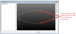
Pick-ups define the position and movement of a variable based on the value of another variable (see Fig. 1). For example, a variable can be defined as a pick-up to maintain a constant thickness in a material or a specific separation between two components.

In some instances, designers may assign too few or too many variables. Though it may seem intuitive to use either simple or complex input criteria, this approach inevitably leads to an insufficient or inordinate number of optimization iterations, while not necessarily producing the best result.

Optimization operands

With an initial design established, designers can then look at adding optimization operands, which are used to define the target or goal of the optimization process. Designers can establish a merit function using numerous different operand types: flux, CIE color coordinates, irradiance, irradiance profiles, intensity, candela or intensity profiles, uniformity, beam width, and user-defined or custom.

Each operand can be used in combination with any other operand. The merit function uses weights to balance the multiple operands based on the desired targets. Additional examples of optimization settings are listed below.

Optimization type: In this instance, downhill simplex is used to allow the optimizer to search through a range of variables.

Characteristic length is used when defining the first simplex when starting the optimization process. Each vertex of the initial simplex is a variable set randomly generated for every variable within its allowed range, hence the characteristic length. Having a fixed random seed number ensures the optimization path is identical and will lead to the same result. If an unrepeatable result is preferred, checking the option of "Generated by timer" would make sure the random sequence is reproduced every time by the system clock.

Stopping conditions determine when the optimization process will be considered finished or complete. Possible stopping conditions include:

• Goal is reached: the process stops when the goal is reached
• Number of iterations: the process stops after a user defined number of iterations
• Iteration tolerance: the process stops when the variation in results from one iteration to the next falls below a certain level

Number of rays traced: One must trace enough rays to get an accurate/stable result in the analysis tools. If too few rays are traced, the graphs can be "noisy" and the results will be difficult for the optimizer to interpret.

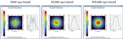
Analyzing the results

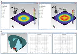
The results of the optimization process can be displayed in methods familiar to optical designers, such as illuminance maps, candela plots, IES and LDT photometric data files, and luminance maps.

Illumination maps show the spatial distribution of light including illuminance, CIE coordinates, and TrueColor. Candela plots show the angular distribution of light; these plots can be used to generate IES and LDT photometric files. These files can then be used in other lighting-design programs such as Dialux, AGI32, and Litestar 4D. The IES and LDT files can also be used to generate custom lighting reports.

Luminance maps show the light from an area that falls in a given solid angle. Commonly used in display and light guide applications. Typical units are candelas per square meter (cd/m²), also called nits. Additionally, certain software programs enable photorealistic rendering that shows how the design will look when manufactured. Photorealistic rending is also useful to see if there is glare or unwanted light visible to the viewer.

Optimization tips

• Start with a good initial design if possible
• Use accurate models, including geometry and properties
• Use accurate source models
• Define enough variables so that the model is not over- or under-constrained
• Set the characteristic length to adequately sample the solution space
• Define achievable optimization operands or goals
• Trace enough rays so that the analysis maps are not noisy and the optimizer can make accurate decisions
• Change optimization parameters to check for better solutions
• Know the capabilities of your optical analysis and optimization software

Since each variable can be visually checked before, during, and after optimization, designers are able to validate the final design iteration to ensure the product's performance requirements can be met quickly and efficiently.

REFERENCES

1. D. Jacobsen, "LED lighting design optimization: Theory, methods, and applications," LED Professional Symposium and Expo (Oct. 2014).

2. See http://bit.ly/1NxraVU.

3. See http://bit.ly/1LIra7Z.

4. See http://bit.ly/1IOyAjP.

5. See http://bit.ly/1JxzzdV.

David Jacobsen is senior application engineer at Lambda Research, Littleton, MA; e-mail: [email protected]; www.lambdares.com.