Photodetector impulse response yields eye-diagram information
The eye diagram of a photoreceiver is a key ingredient in assessing performance of an optical-communications network. A practical method derives the eye diagram from the measured impulse response of a photodetector.
The eye-diagram transmission pattern is a critical and commonly used measure of optical-link performance in optical networks. The eye diagram of the photoreceiver or photodetector, in particular, is a key element in determining the link budget. However, deconvolving the eye-diagram response of the photodetector from that of the source and performing such measurements at varying frequencies can be difficult or nearly impossible, especially at higher data rates such as 40 Gbit/s.
We have devised a method for deriving an eye diagram from the measured impulse response of photodetectors and have compared results from this approach with measured eye diagrams. By determining and comparing eye diagrams for a wide range of photodetectors, we have demonstrated and quantified how features of the impulse response influence the eye opening. The method, in consideration with important factors such as noise-equivalent power of the receiver, is helpful in modeling and diagnosing receiver behavior.
Pulsed-laser measurements
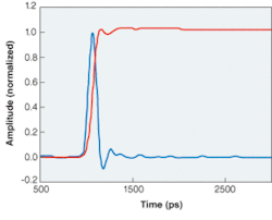
For a linear receiver, the impulse response contains all the information about its behavior (neglecting noise for now), and therefore can be used to calculate its eye-diagram shape. The impulse response is best measured by a system with a bandwidth much higher than the receiver itself. A subpicosecond modelocked laser is sufficiently fast for even the fastest receivers, and a 50-GHz oscilloscope will work well for receiver bandwidths up to 15 or 20 GHz. With such a pulsed-laser measurement setup, the 23-ps full-width at half-maximum (FWHM) pulse of a 15-GHz receiver would only broaden to 24 ps.
One important consideration in such measurements is the optical saturation level of the receiver under pulsed-laser excitation. Saturation will begin when the output signal reaches a certain level, and for all signal types (including pulses) this level is given roughly by the continuous-wave (CW) input saturation power (PCW) multiplied by the gain, G. For pulses much shorter than the response time of the receiver the output pulse will have a width equal to the FWHM of the receiver’s impulse response.
For pulses of period T, then, the average power at saturation will be PCW scaled by the duty cycle of the output signal, FWHM/T. For example, a 1-mW, 10-MHz laser used with a 10-GHz receiver (35-ps FWHM) with PCW = 1 mW would need to be attenuated by a factor of 35 × 10-12/100 × 10-9 or 35 dB.
A second consideration of pulsed-laser measurements is offsets that might result from the oscilloscope or a DC-coupled receiver. Because a data sequence can have long strings of zeros and ones that approximate step functions and the integral of the impulse response is the step function, the cumulative effect of integrating with even a small offset present produces significant errors. For this reason, it is important to subtract offsets from the impulse measurement, which can be accomplished by subtracting the average background signal level taken over some window prior to pulse arrival from the entire measured impulse (see Fig. 1).
Deriving the eye diagram
The receiver’s response to an input data stream is the convolution of its impulse response with the input data signal. One approach to this calculation might be to take a chosen bit pattern, convolve it with the impulse response, and then superimpose all of the bits in a single plot. Such a method would allow the extraction of statistical information (for example, signal-level distribution at a given point within the bit period) but could prove cumbersome-to test all possible bit patterns in an N-bit word would require 2N convolutions.
An alternative approach is direct calculation of the smallest envelope into which an eye diagram would fit. Such an envelope represents the bounds for all possible bit patterns of a given length and hence can be thought of as the worst-case eye. While the method (described below) does not provide statistical information, it is nonetheless useful in that it enables designing for the worst-case scenario.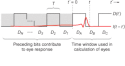
To see how this envelope is calculated, consider a NRZ (non-return-to-zero) bit pattern of length N + 3 (see Fig. 2). Performing the 2N+3 convolutions and superimposing bits A, B, C for each would lead to an eye diagram, and the convolutions would be:
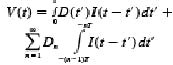
where V(t) is the voltage at the output of the receiver, D(t) is the input data (zero rise-time assumed), I(t) is the receiver impulse response, Dn are either +1 or -1, the first term is due to bits A, B, C, and each term of the summation is the contribution from the nth preceding bit. When the pattern defined by Dn is such that all terms of the summation are positive, the summation then represents a maximum contribution to V(t). Adding and subtracting (for the complementary pattern) this value to the eight patterns possible with bits A, B, C and superimposing the resulting 16 V(t)s leads to an eye, the envelope of which is the sought-after worst-case eye:
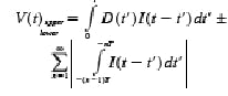
Calculation of V(t) is quite manageable even for long sequences exceeding 32 bits. Note that the sign of the term in the absolute value tells you whether bit nshould be high or low to produce the maximum or minimum contribution-thus the impulse response can also be used to predict problematic data patterns.
It is worth mentioning that for a finite impulse measurement window, the impulse response must be zero outside of the window. Also, note that the length of the measurement window determines the total pattern length for the resulting eye. Thus, a window that accommodates 31 bits is not the same as a 231 - 1 PRBS (pseudo-random bit sequence), but provided the impulse response is zero outside of the window, then the resulting eye should be valid. If one wishes to model a receiver whose response has very long time components, then additional worst-case assumptions can be made that enable calculation of the eye. In this case frequency-domain or step-response measurements are useful, but beyond the scope of this article.
Derived vs. measured
Using the 4-GHz receiver whose measured impulse and step responses are shown in Fig. 1, we derive the eye diagram shapes using the method described above for 2.5, 5.5, and 8.5 Gbit/s data rates (see Fig. 3, left). As expected, the method predicts a narrowing of the eye opening with increased bit rate.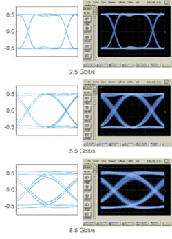
The same 4-GHz receiver was measured at 2.5, 5.5, and 8.5 Gbit/s using a 12.5-GHz pattern generator with a near-ideal transmitter (a DFB laser with a 12-GHz lithium niobate Mach-Zehnder modulator). The measured eye diagrams use NRZ data in the form of a 231 - 1 PRBS (see Fig. 3, right). The calculated eye diagrams demonstrate good overall agreement in eye shapes to the measured eyes. Some minor discrepancies are apparent such as the “splitting” in the measured rising and falling edges at the higher bit rates.
Time response dictates eye-diagram shape
Using this approach, we compared the eye diagram at varying bit rates of various high-speed detectors. We found that the time-domain response of a detector dictates the eye-diagram shape and that optimizing the detector for the proper time-domain response can result in clean eye openings.
In particular, we compared two 20‑GHz photodetectors, one with a slight tail in the impulse response and one optimized for time-domain performance that does not exhibit a tail (see Fig. 4, left). Using these impulse responses and the approach described above, we derived the eye diagram at 20 Gbit/s for these two detectors (see Fig. 4, right). The eye opening of the detector with the slight tail is significantly worse than that for the detector optimized for time domain. Thus, even slight changes in the time-domain response can have dramatic effects on the eye diagram.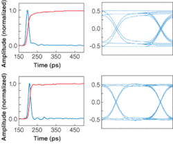
Responsivity and noise
Although the method described above provides an accurate picture of eye-diagram shape, it does not take noise into account. Noise broadens the traces of the eye diagram and reduces the eye opening by introducing statistical variations into the eye response. The detector noise is commonly characterized by its noise-equivalent power (NEP), which is determined primarily by the detector responsivity and amplifier noise. Detectors optimized for low NEP as well as optimal time-domain response can therefore result in maximum eye openings (see Fig. 4, bottom left and right).
Using this method, we have evaluated many high-speed detectors without the need for costly high-speed (20- or 40‑GHz) bit-error-rate testers. We have found that even small changes in the time-domain response can have dramatic effects on the eye-diagram response and that detectors optimized for time-domain operation can exhibit optimized eye-diagram response. While this method does not fully substitute for true bit-error-rate testing and eye measurement, it does provide an effective means for detector characterization and optimization for communications applications.
About the Author
Herman Chui
Vice President & General Manager, MKS Spectra-Physics
Herman Chui is Vice President & General Manager, Photonics Solutions Division, Lasers at MKS Spectra-Physics (Milpitas, CA).
Andrew Davidson
Senior Staff Engineer, MKS Newport - New Focus
Andrew Davidson is a Senior Staff Engineer at MKS Newport - New Focus (Irvine, CA).