SURFACE CHARACTERIZATION: Surface qualification demands a proper measurement technique
DAVE CHANEY, JOHN FLEMING, FRANK GROCHOCKI, AND MICHAEL DITTMAN
The characterization of optical surfaces is critical to assessing the performance of an optical system prior to system integration. Knowing what characterization needs to be performed is dependent on a detailed understanding of requirements. Once requirements are well understood and flowed down to individual optical components, specifications for the individual optics can be determined. These specifications can cover a wide range of spatial frequencies and the measurements required to confirm compliance can involve very different techniques.
There is no set definition of low-, mid-, and high-spatial-frequency errors; however, measurement of low-spatial-frequency errors or surface-figure errors is usually required to assess the image quality of the optic and the system. With spatial-frequency ranges generally less than 1 cycle/mm, these errors are typically assessed with interferometric systems. Mid-spatial-frequency errors cover the range of angles just outside the first couple of rings of the point-spread function (PSF) to spatial frequencies that equate to scatter angles of a few degrees. Spatial-frequency ranges are typically from 0.2 to 20 cycles/mm. High-spatial-frequency errors are typically the domain for scattered-light calculations and are usually measured through bidirectional scatter-distribution-function (BSDF) measurements and optical profilometry. Spatial-frequency ranges for these measurements are generally greater than 10 cycles/mm. An understanding of each measurement and its shortcomings is critical to an accurate assessment of the optical performance.
Surface-figure characterization
The surface figure of an optic is defined as the perturbation of the optical surface from the perfect optical prescription. While surface figure has typically referred to low-frequency errors, the past several years have seen the definition broaden to include mid-frequency errors. This is because both frequency regions will affect system performance, though differently, and therefore must be controlled.
Low-frequency errors tend to transfer light from the center of the airy disk pattern into the first few diffraction rings. This effect reduces the magnitude of the point-spread function without widening it, thus reducing the Strehl ratio. Mid-frequency errors or small-angle scatter will widen or smear the PSF and reduce contrast.1, 2 Low-frequency and mid-frequency errors can both degrade the optical system performance and are frequently measured to ensure specifications are met. However, some figure imperfections can be omitted from a surface-figure specification. This is often the case for power and occasionally astigmatism. Many optical systems allow the individual optics to be focused, decentered, or tilted to compensate for specific aberrations. Relaxing requirements by incorporating these compensations in the system-level error budget will increase the manufacturability and reduce the costs of the optical components.
The surface figure of an optic is measured through a variety of means. Two common methods of testing optics use either a coarse-figure profilometer or an interferometer. The former is a simple approach of actually touching or dragging a probe over an optic to measure the profile or surface height at discrete points. This method is commonly done using a coordinate measuring machine (CMM) for larger optics and custom profilometers for smaller ones. The height information is processed to generate a three-dimensional (3‑D) surface map. A major advantage of this method is its ability to measure aspheric optics without the use of complicated test setups or additional null optics. On the other hand, disadvantages include limited accuracy and spatial resolution (not a good choice for measuring mid-frequency errors). It is, however, an excellent method if the figure tolerances are relatively loose or if it is used to manufacture the optic to the point at which it can be tested optically. This is where interferometric testing takes over.
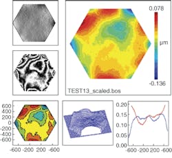
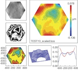
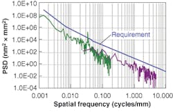
The interferometer generates and splits a test beam into two components-test and reference wavefronts-and then recombines them, typically on a CCD for fast data processing. Deviations in the optical surface are seen as a phase change in the wavefront at a given pixel. When the phases of all pixels are calculated, a map of the surface figure can be generated. Phase shifting, either temporally or spatially, is used to increase the optical path length of either the test or reference arms. This technique greatly reduces the data-processing time and is used to determine signs of perturbations. Low-spatial-frequency errors measured on an optic can be plotted using an interferometer, converted to power-spectral-density (PSD) space, and compared to a derived requirement (see Fig. 1 and Fig. 2). While interferometry offers many advantages, including speed, accuracy, and spatial resolution, it also has disadvantages: the need for null lenses or diffractive nulls when testing aspheric optics and sensitivity to vibration and other environmental effects.
Surface figure is specified on optical drawings or specifications. The terminology used is often dependent upon the frequency band of the error to be controlled. Low-frequency errors are typically specified as irregularity, fringes of departure, or flatness. Mid-frequency errors are specified using slope or PSD requirements. Finally, surface accuracy and surface figure are terms often used to capture both regions. Waves are the predominant unit value used in specifications; however, care must be taken to include the wavelength of interest. To eliminate ambiguity, it is better to use microns or nanometers as the unit value in specifications. Confusion in the specification can still exist if root-mean-square (rms) or peak-to-valley (PV) is not explicitly stated.
The magnitude of the requirement is derived from experience or optical-system modeling. Common software tools used for optical modeling include CODE V from Optical Research Associates (ORA; Pasadena, CA), ZEMAX from Zemax (Bellevue, WA), and OSLO from Lambda Research (Littleton, MA). All of these programs have methods to tolerance surface figures of the individual elements, though tolerancing low-frequency errors is much easier than mid-frequency.
Phase-measuring microscope profilometry
As surface figure is vital to the optical designer working in the lower-spatial-frequency regime, knowledge of surface microroughness is critical to the stray-light analyst working in the higher-spatial-frequency regime. Optical profilometry can be performed to characterize the root-mean-square roughness of an optical surface. However, the measurement of surface roughness is inherently bandwidth limited and is prone to instrumental effects.3 The spatial frequencies that can be measured vary with the magnification used and these multiple measurements must be corrected properly before converting to a BSDF and comparing to stray-light requirements.4, 5
To get good correlation it is necessary to correct the profilometry for instrumental errors and to perform azimuthal averaging on the 2-D PSD. Without such corrections, measurements of surface roughness from the profilometer can be highly inaccurate. Surface-roughness requirements need to be rigorously flowed down from stray-light requirements and compared over agreed-upon spatial frequencies. A single value for root-mean-squared roughness with no corresponding spatial frequency range is insufficient for an optic.
BSDF
Measurements of bidirectional scatter-distribution function are used to assess the scatter of an optical surface from about 0.5° from specular out to grazing scatter angles. The BSDF is the ratio of the surface radiance to the input surface irradiance. The scatter measured at a specific angle can then be converted to PSD space. At visible wavelengths these spatial frequencies are on the order of 10 cycles/mm to the wavelength being used in the measurement. These measurements are vital for assessing the stray-light performance of an optical system. Vendors for scatterometer instruments are Schmitt Industries (Portland, OR) and Surface Optics (San Diego, CA). Smaller handheld instruments are available, but are typically not accurate enough for low-scatter optical components.
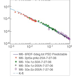
To show that these measurements are consistent and demonstrate the process for using an optical profilometer to measure surface PSDs and predict their BSDF characteristics, a series of profilometry measurements at several magnifications were taken with a Zygo (Middlefield, CT) NewView profilometer and were corrected and converted to PSD space. These were compared to a BSDF measurement taken at 633 nm with a Schmitt scatterometer and also converted to PSD space (see Fig. 3). Although the BSDF instrument is unable to measure spatial frequencies lower than about 0.05 cycles/mm, profilometry can be used to predict the scatter at very small angles.
A cautionary note
Optical profilometry can generally be performed faster than BSDF measurements and vendors can verify a surface-roughness requirement much more easily than a BSDF requirement. Once properly corrected for measurement errors, profilometry can be used to accurately predict the scatter properties of an optic. In addition, optical profilometry covers mid- and high-spatial-frequency errors and thus can be used to predict scatter at very small angles from specular. These small-angle scatter measurements (less than 0.1° from specular) cannot be performed with available BSDF instruments. Extreme care must be taken to ensure that the profilometry data is properly corrected before they are used to predict the scatter from the surface. Both optical profilometry and BSDF measurements are generally performed on small areas of a surface and do not characterize the entire surface.
Measurements of surface-figure errors can be performed over large areas of an optic and thus give a more complete assessment of the optic. In addition, the latest instruments provide accurate information well into the mid-spatial-frequency range and thus can also be compared to microscope profilometry.
Once the PSD of a surface is known, it can be used to predict the scatter at theoretically any wavelength. However, surface profilometry is not the only cause of scatter from an optic. Particulate and molecular contamination can cause significant additional scatter and this is very difficult to predict precisely for the integrated optical assembly. Scaling the PSD into the infrared is also incorrect in predicting scatter performance for many materials because at longer wavelengths the scatter is no longer due solely to the surface topography. Taking BSDF measurements at wavelengths where the optic is used and performing system-level stray-light modeling and testing are often the only means to ensure these requirements are met.
REFERENCES
1. Harvey et al., Proc. SPIE 2576-25 (1995).
2. M. Bigelow and N. Harned, OE Magazine (November/December 2004).
3. Dittman et al., Proc. SPIE 6291, 62910P, 1 (2006).
4. E.L. Church and P Z. Takacs, Proc. SPIE 1009, 46 (1988).
5. E.L. Church and P.Z. Takacs, Proc. SPIE 1164, 46 (1989).
DAVE CHANEY, JOHN FLEMING, FRANK GROCHOCKI, and MICHAEL DITTMAN are optical engineers at Ball Aerospace & Technologies, 1600 Commerce St., Boulder, CO 80301; e-mail: [email protected]; www.ballaerospace.com.